Predictive Analysis Model to Forecast Quantity Demand

Background:
In early 2021, I worked on a project with one of the most popular outwear companies. The project objective was to deal with continuous occurrences of customer orders getting canceled or delayed simply due to a lack of supply; in fact, in the previous season itself, over half of the orders placed were either delayed or fell short due to this very reason. Throughout the project, I was working closely with fellow data scientists, data analysts, business analysts, as well as the internal business stakeholders of the demand and supply department within the organization.

Solution:
As we conducted numerous research and explored various avenues, we decided that the best course of action would be to project the number of units demanded utilizing predictive modeling. The plan is to foresee the clothing styles (products) that are expected to run out of inventory by comparing the quantity available against its demand-forecasted units. By extracting this piece of information, we would then be able to place blind buys from our respective vendors accordingly ahead of time for those expected supply shortages and prevent orders from getting canceled or delayed due to this very reason.
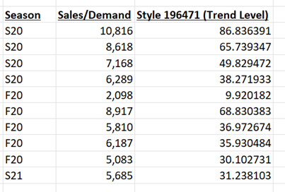
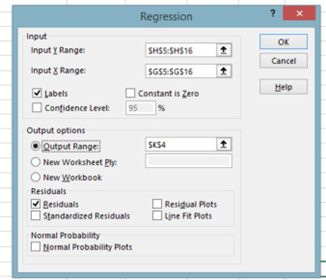
To begin with, we had created a user-defined function in SQL Server that calculates a “Trend Level”. This trend level is a numerical calculated measure that takes into consideration various factors (such as marketing/advertising expenses, merch judgment, etc) and returns a single value that is associated with a single clothing style line item. We then initially proceeded to build a predictive analytical model utilizing Microsoft Excel’s multiple linear regression tool, using Trend Level as our independent variable to project the demand forecast units.

(All screenshot uses dummy/mock dataset)




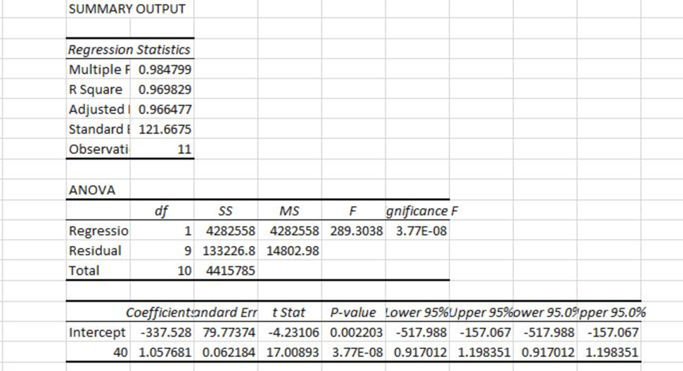
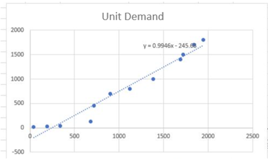
We encountered issues when utilizing a combined single feature, 'trend level,' which resulted in a significantly high R-squared value close to 1. To address this, we adopted an alternative approach by treating the factors as separate and independent variables, resulting in a total of 7 features. Leveraging the PySpark machine learning library, we employed a comprehensive pipeline that included OneHotEncoder, StringIndexer, VectorAssembler, StandardScaler, and LinearRegression to construct and train our linear regression predictive model. In this process, we initiated feature selection, performed scaling, split the dataset into test and train samples, and fitted the model using linear regression. Subsequently, we generated predictions and assessed the model's performance and accuracy using Root Mean Squared Error (RMSE) and R-Squared metrics. Please find a sample of the code below.

#Scaling features
# Initialize the `standardScaler`
standardScaler = StandardScaler(inputCol='features', outputCol='features_scaled')
# Fit the DataFrame to the scaler
scaler = standardScaler.fit(transformed_df.select('features'))
# Transform the data in `df` with the scaler
scaled_df = scaler.transform(transformed_df)
scaled_df.select('features', 'features_scaled').show(5, truncate=False)

#Create Test/Train Split
train_data, test_data = modeling_df.randomSplit([0.7, 0.3],seed=1234)
train_data.show(5, truncate=False)

#Fitting Linear Regression Model
lr = LinearRegression(labelCol="label", maxIter=100, regParam=0.3, elasticNetParam=0.8)
linearModel = lr.fit(train_data)

#Make Predictions
predicted = linearModel.transform(test_data)
predicted.select('label', 'prediction').show(5)

#Evaluating the Model
linearModel.summary.rootMeanSquaredError
linearModel.summary.r2

scored_df = predicted.select('label', 'prediction').toPandas()
scored_df.rename(columns={'label': 'Quantity_Demanded', 'prediction': 'Quantity_Demanded_Predicted'}, inplace=True)
_ = sns.lmplot(x='Quantity_Demanded', y='Quantity_Demanded_Predicted', data=scored_df, height=6, aspect=1, fit_reg=True)

Conclusion:
By utilizing the data extracted from regression model, we were able to successfully improve margin dollars. Overall, we experienced a 13% increase in on-time orders compared to the previous season. Furthermore, orders delivered past the cancel date have dropped by 17%, followed by only 4% of customer orders that ran out of supply.
I would like to express my gratitude to Columbia Sportswear for this amazing opportunity and experience. I would also like to thank the amazing individuals who were apart of the project over at Columbia and prAna from the engineers, to the analysts, to the stakeholders.